Brockhouse - Wiggler Low Energy Beamline
Overview
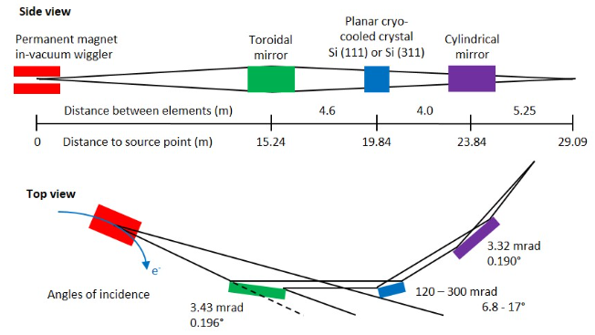
The optical configuration of the Wiggler Low Energy (WLE) beamline consists of an in-vacuum wiggler, a toroidal mirror, a single side-bounce Bragg monochromator, and a cylindrical mirror. The beamline produces a sub-150 um V x 500 um H focused beam on the order of 1012 photons/s at the sample. Three endstations operate in a spacious hutch at fixed photon energies.
Beamline technical details and performance
Click here for a pdf copy of the WLE beamline paper
Leontowich, A. F. G., Gomez, A., Moreno, B. D., Muir, D., Spasyuk, D., King, G., Reid, J. W., Kim, C. Y., and Kycia, S. ‘The lower energy diffraction and scattering side bounce beamline for materials science at the Canadian Light Source.’ J. Synchrotron Rad., 28 (2021) 961-969
| Energy range: | 7 – 22 keV |
|---|---|
| Flux, @ 220 mA, minimum gap: | 10¹² photons/s with Si(111), or 10¹¹ photons/s with Si(311) |
| Beam size, FWHM: | Better than 150 μm V × 500 μm H |
| Energy resolution, ΔE/E: | 2.5 – 6.4 × 10⁻⁴ |
| Divergence: | 200 – 300 μrad V × 730 μrad H |
High-Resolution Powder X-ray Diffraction (PXRD)
This endstation operates at a fixed photon energy of 15132.0 eV (λ = 0.81935 Å), using the Si(111) crystal in the beamline monochromator. There are eight Dectris Mythen2 X series 1K "linear strip" detectors. Each has 1280 pixels, which are 8 mm wide by 50 μm tall, for a total active area of 8 mm × 64 mm per detector. These are direct detection with 1 mm thick silicon as the sensor. The response is linear up to 700,000 counts/s, with practically no dark noise, and an acquisition rate of up to 1000 Hz.
The detectors are 760 mm from the sample and spaced 10º apart. For typical data collection, 2θ is scanned 10º, (from -7° to 3°, with 2θ = 0° defined as the center of the lowest angle detector) acquiring every 0.25º for 2 seconds. This effectively collects a 2θ range of 1.35° - 75.0°, which is a q range of 0.18 Å-1 - 9.32 Å-1, or a d spacing range of 34.8 Å - 0.67 Å. Samples are spun at a rate of 2 Hz during measurement. A fast shutter is synchronized to the detector acquisition to minimize the radiation exposure. The full measurement cycle (transfer on - align - measure - transfer off) is 4 minutes 30 seconds per sample.
This endstation can be paired with the Oxford Cryostream 800 Plus for temperature control (80 - 500 K). Please give advanced notice as the Cryostream is a shared resource within the BXDS sector.
When writing a PXRD proposal, estimate 2 hours for initial instrument setup and calibration, and 10 minutes per sample at room temperature. If temperature control is required, mention you require the Oxford Cryostream for temperature control, and also include details of what temperatures you want, and any temperature ramps.
PXRD sample preparation and shipping ***PLEASE READ***
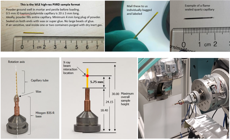
New sample prep video here, but please also read these written instructions
Users are responsible for all sample preparation. Please prep all samples as detailed below before your scheduled time.
1) Purchase some capillaries: Users will purchase their own capillaries, and pack their powdered samples into capillary tubes. Standard capillaries for this endstation are polyimide/Kapton, 0.5 mm inner diameter. These capillaries are sourced from VWR, part MFLX95820-04. Samples that are not compatible with Kapton can be loaded in quartz capillaries and flame sealed. These can be purchased as a custom order from Friedrich and Dimmock: 0.5 mm ID, 0.7 mm OD, 75 mm total length.
2) Consider sample absorption: For each sample, users must calculate the sample absorption in the form of a µR value (where µ is the linear absorption coefficient, and R is the capillary radius) at our wavelength of 0.81935 Å. You can use this APS web calculator, https://11bm.xray.aps.anl.gov/absorb/ , or the free program MAC 3.0 for the calculation. It can be downloaded here.
- Type in the unit cell and press the Calc Vol button.
- Type in the elemental formula, and press the Load Form button. The estimated number of formula units (Z) should be close to the correct value, but change it to the exact value.
- Press the Calc Density button.
- Type in either the energy or wavelength for the experiment and press the appropriate Convert button to calculate the wavelength or energy.
- Type in the radius of the capillary for the experiment (not the diameter) and press the Calc MAC button. The PXRD mu*R will be calculated.
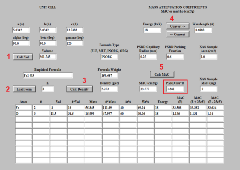
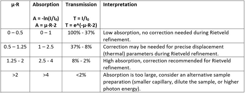
If the calculated µR value is >2 in a 0.5 mm capillary, consider switching to 0.3 mm ID capillaries (VWR, part MFLX95820-02) , or diluting the sample (this idea goes at least as far back as B.D. Cullity, Elements of X-ray Diffraction, 2nd ed., 1978). Crushed up fused silica or borosilicate glassware works well for diluting samples. Dilute highly absorbing samples so that the µR is less than 2. Dilution up to a factor of 16 has been successful. A factor of 20 was found to be too dilute.
3) Prepare a nice powder: Large grains will reduce the quality of the data. If the sample is a mixture, and the mixture is not homogeneous within the beam area (150 µm V × 450 µm H FWHM), the phase fractions measured will not be reproducible. The solution is to grind samples well with a mortar and pestle (or mechanically micronized, if possible) to a crystallite size on the order of 1 µm, provided this can be completed without inherently damaging the sample. Mineralogical and inorganic materials samples can generally (but not always) be grinded or micronized to reduce crystallite size without significantly changing other properties of the sample (like the crystallographic phase observed or the phase composition of multiphase mixtures). Conversely, pharmaceutical and organic samples are often more sensitive to grinding, which may induce phase changes to new crystalline polymorphs, undesirably produce nano-crystalline size or transformation to an amorphous phase.
4) Fill and seal the capillaries: Proper size and sealing is important: The capillary should be 20 +- 3 mm long. Pack the powder in to create a plug of material at least 5 mm long (preferably as full as possible). You can use a small diameter wire, or small diameter Kapton capillary to pack powder into the capillary. Kapton capillaries must be sealed on both ends so the powder stays in the tube. Use wax, superglue, or modelling clay for sealing. Samples which are very air-sensitive can be prepared in a glovebox and sealed on both ends with 5 minute epoxy (see some tips here). Take care not to form a bead of glue at the end which is wider than the capillary, or it may not be possible to fit it in the magnetic stub holder. If the sample is air-sensitive, ship it within one or two air-tight containers purged with dry inert gas (for example, a capillary in a small glass vial inside a small plastic bag). These packages can be opened at the beamline immediately before the data collection.
5) Mail your capillaries to us, or come visit! Users no longer need to come on site for ordinary measurements of powders in capillaries at ambient conditions. If the experiment is something out of the ordinary, you may need to visit to complete your experiment. The mailing address for your sample shipment is,
Canadian Light Source
Attn: Adam Leontowich, Project: (Write your project number here)
44 Innovation Blvd
Saskatoon, Saskatchewan
S7N 2V3
Canada
Please do not wait until the very last minute to mail your samples, especially when shipping to us from outside Canada.
The sealed capillary is then mounted on a reusable magnetic stub with a small amount of wax. The magnetic stubs are from Mitigen, Goniometer Base Type B3S-R, GB-B3S-R-40. We will provide the stubs for users. We generally do not mail stubs or capillaries to users. You send or bring the pre-prepared capillaries, which are mounted to stubs on-site. During sample mounting, the capillary needs to be pre-aligned by eye to be colinear with the rotation axis of the stub. Samples are measured while spinning at 2 Hz. Rotational wobble of the sample greater than 0.5x the capillary diameter has a significant effect on peak shape (Bergamaschi et al., JSR, 17, 653 2010) . The capillaries are measured oriented horizontally at a slight downward angle of 2° while spinning. The slight angle prevents loose powder particles from moving out of the beam during measurement.
For best results, we encourage users to,
- Prepare all samples in capillaries ahead of the scheduled beamtime, as detailed above.
- Create a priority list. Ensure that your most important measurements get done first in case there are unexpected problems.
- Use a very simple naming convention for your samples (A1, A2, A3, B1, B2, C1, etc.). This makes it much easier for staff who receive hundreds of samples a week.
PXRD data format and how to view your data
When you receive your data we will typically include three types of files:
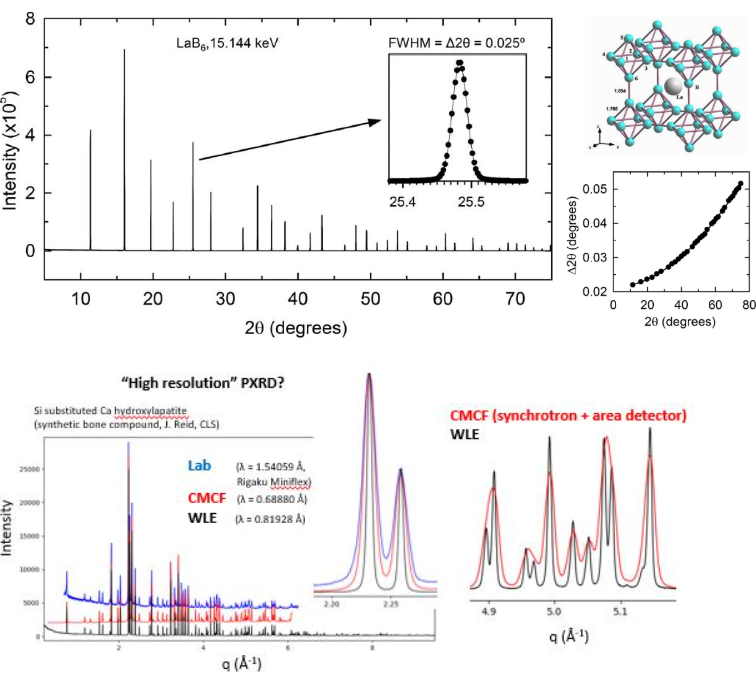
- Files with the extension .xye are the important PXRD data. The format is essentially that of TOPAS data with no header. The first column is 2θ, the second column is intensity in counts/s, and the third column is error. PyMCA is a free program also useful for quickly viewing the patterns. We use the free program GSAS-II for most PXRD data workup. These files open in GSAS-II (import, powder data, guess format from file). When it asks for an instrument parameter file, load in the BXDS_Huber.instrprm file available below for dowload. Now the data file should open. By refining the data for the calibration standard LaB6, using the .cif file for LaB6 available for download below, you can create, save, and apply your own instrument parameter file to the data.
- The files with no extension are the individual frames from the scan, and can be viewed with PyMCA. These frames get merged together to form the .xye files. Typically users will not need these, but they can sometimes be useful.
- Lastly, there are files that end in _spec. These contain additional information collected during the scans, such as ion chamber readings and the ring current for each point in the scan.
Click here to download a collection of helpful PXRD files
- A GSAS-II instrument parameter file specific for the Huber endstation (last updated Oct. 28, 2025)
- Example of a .xye file for LaB6 (NIST 660b)
- Example of the MAC program with details entered for LaB6, courtesy of Joel Reid
- .cif file for LaB6
- Information from NIST on the LaB6 calibration sample (NIST 660b)
- A step-by-step tutorial for how to refine LaB6 in GSAS-II, courtesy of Joel Reid
Publishing PXRD data
The following statement is typically adequate for the experimental section of your manuscript. Note that the information in bold might be different for your experiment,
Samples were loaded into 0.5 mm diameter Kapton capillaries and rotated at 2 Hz during the measurement. Powder patterns were measured at 298(1) K at the Wiggler Low Energy Beamline (Leontowich et al., 2021) of the Brockhouse X-ray Diffraction and Scattering (BXDS) Sector of the Canadian Light Source (CLS) using a wavelength of 0.81935 Å (15.1 keV) from 1.6 - 74.9° 2θ with a step size of 0.0025° and a collection time of 3 minutes. The high resolution powder diffraction data were collected using eight Dectris Mythen2 X series 1K linear strip detectors. NIST SRM 660b LaB6 was used to calibrate the instrument and refine the monochromatic wavelength used in the experiment.
[1] Leontowich, A. F. G., Gomez, A., Moreno, B. D., Muir, D., Spasyuk, D., King, G., Reid, J. W., Kim, C. Y., and Kycia, S. ‘The lower energy diffraction and scattering side bounce beamline for materials science at the Canadian Light Source.’ J. Synchrotron Rad., 28 (2021) 961-969.
Also, CLS requires this standard funding acknowledgement within the paper,
“Part or all of the research described in this paper was performed at the Canadian Light Source, a national research facility of the University of Saskatchewan, which is supported by the Canada Foundation for Innovation (CFI), the Natural Sciences and Engineering Research Council (NSERC), the Canadian Institutes of Health Research (CIHR), the Government of Saskatchewan, and the University of Saskatchewan.”
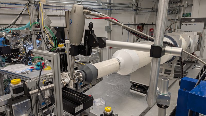
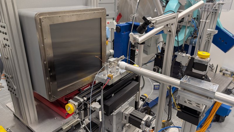
SAXS/WAXS
We recently completed a new table and detector bracket that enables a faster reconfiguration between SAXS and WAXS modes.
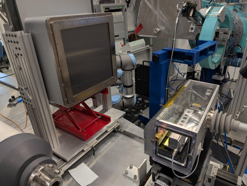
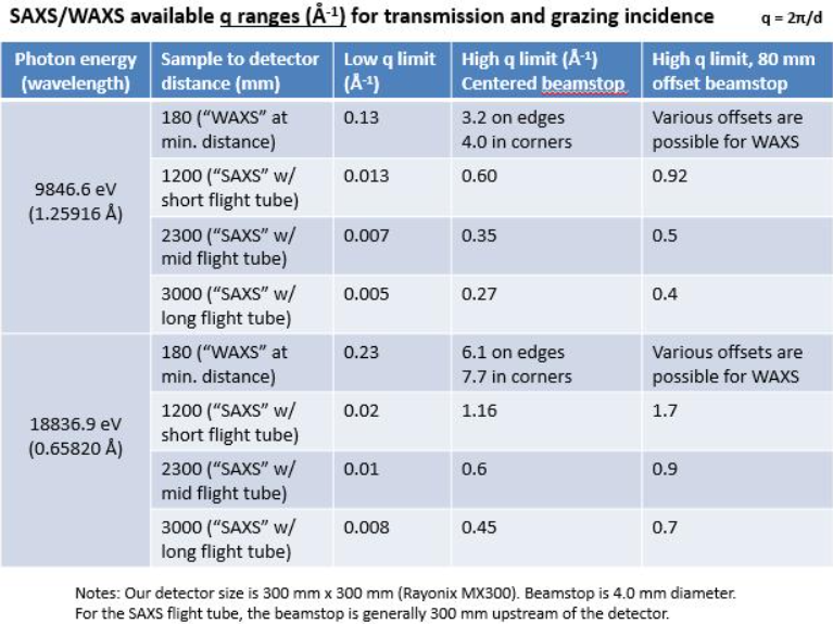
This endstation has a choice of two fixed photon energies: 9871.3 eV (1.25602 Å) with Si(111), or 18883.3 eV (0.656586 Å) with Si(311). 9.9 keV is generally better for measuring in grazing incidence geometry, SAXS of liquids, reaching our lowest possible q value for SAXS, and organic materials. 18.9 keV is generally better for transmission through thick and dense materials, reaching the highest possible q value for WAXS, and inorganics such as battery or perovskite materials.
The detector is a Rayonix MX300 phosphor coupled CCD. The area is 300 mm × 300 mm, with minimum pixel size of 73.242 μm × 73.242 μm (4096 × 4096). The acquistion rate can be as fast as 2 Hz, in 4×4 binning mode. The maximum counts per pixel is 2^16 = 65536. The beamstops which protect this detector are 4.0 mm diameter with an embedded photodiode.
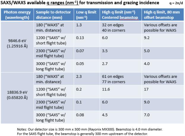
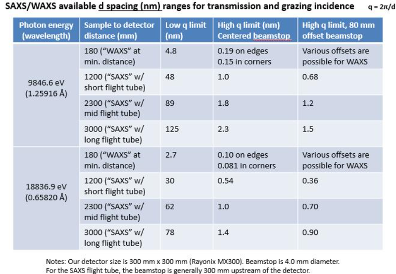
A variety of q ranges are possible, and these configurations are listed below in units of inverse angstroms and nanometers.
We use a four stage stack for sample manipulation. Measurements can be performed in transmission or grazing incidence geometry (minimum θ step = 0.01º). The endstation can be paired with a several special environments available at the beamline:
- Multi-sample holders for transmission or grazing incidence measurements
- Oxford Cryostream (80 - 500 K)
- Linkam heating/cooling stage suitable for grazing incidence (77 - 623 K)
- High temperature furnace with gas flow (up to 1473 K)
- In-situ spin coater
- Liquid flow cell and syringe pump
- Helium atmosphere boxes (one single sample that accommodates the Linkam stage, and one multi-sample) for ultra-low background WAXS.
We are also open to putting your device in the endstation! We have accommodated user-designed tensile stages, heating stages, solar simulators, humidity control, etc. Contact staff well in advance when requesting a special sample environment.
We can measure powders, thin films. liquids, pharmaceuticals, nanoparticles in solution or on surfaces, micelles... the list goes on! For liquids, we generally need minimum 40 uL for the measurment. SAXS of liquids requires concentrations of 1 - 10 mmol, or about 1 - 10 mg/mL, if you are interested in the form factor. Liquid samples are measured in quartz capillaries (buy the 1.5 mm, no funnel, open on both ends, part Quartz 15-SQZ - 1.5mm), and users are expected to bring their own capillaries. We supply silver behenate and LaB6 (NIST 660b) for the detector calibration, and glassy carbon (NIST 3600) as an absolute intensity standard.
For best results, we encourage users to,
- Let us know in advance the q (Å-1) or d spacing (Å) range you are interested in. We can optimize the setup for your specific problem. Our currently available q ranges are tabulated above.
- Create a priority list. Ensure that your most important measurements get done first in case there are unexpected problems.
- Use a very simple naming convention for your samples (A1, A2, A3, B1, B2, C1, etc.). This makes it much easier for staff who receive hundreds of samples a week.
- For a SAXS/WAXS proposal, include 2 hours of initial setup time. Due to the wide variety of samples we see, sample throughput could be between 1 and 30 minutes for a sample at ambient conditions. Consult with beamline staff. The processes of 1) switching from SAXS to WAXS, 2) changing the photon energy, or 3) changing the flight tube length, all require about 2 hours of setup time, and are performed by beamline staff. Please tell us if you plan any configuration changes ahead of your visit. They must start and conclude within the hours of 9 am - 4 pm, Monday to Friday. After hours and weekends may be possible with advanced notice. We have kids :) Asking for a configuration change at 3:30pm that takes 2 hours will likely be declined.
SAXS/WAXS data format and how to view your data
Data from the Rayonix detector are images in the .tif file format, 33 MB in size. The free program ImageJ is installed at the beamline for a quick visual check of the image quality.
We use the free program GSAS-II for some SAXS/WAXS data workup. The .tif files open in GSAS-II (import, image, from TIF image file). Now the data file should open. By refining the data for the calibration standard such as silver behenate or LaB6, you can calibrate the detector, and then apply the calibration to your data to perform azimuthal integrations in units of q. GSAS-II also has excellent tutorials which fully describe these steps (click help, tutorials, browse tutorial on web, "calibration of an area detector", and "integration of area detector data").
New SAXS data workup videos!
Part 1: SAXS data calibration and reduction using GSAS-II
Part 2: SAXS data manipulation and analysis using BioXTAS RAW and SASView
- BioXTAS Raw is excellent for SAXS analysis (Guinier, Kratky, PDDF).
- GIXSGUI is popular Matlab based program for more advanced GIWAXS data workup including creating missing-wedge figures.
- BornAgain is excellent for modeling and analysing GISAXS data.
Publishing SAXS/WAXS data
The following information is typically adequate for the experimental section of your manuscript. Note that the information in bold might be different for your experiment,
"SAXS-WAXS experiments were performed at the Canadian Light Source (CLS) synchrotron using the Brockhouse X-ray Diffraction and Scattering (BXDS) sector Wiggler Low Energy (WLE) beamline [1]. The photon energy was 9871.3 eV selected using a Si(111) monochromator. Diffraction patterns were collected with a Rayonix MX300 CCD detector (300 mm × 300 mm active area with 73.242 μm × 73.242 µm pixels). The sample to detector distance was 2337 mm for SAXS and 293 mm for WAXS, with both configurations using a 4.0 mm diameter beamstop. The data were calibrated using silver behenate (SAXS) and NIST 660b LaB6 (WAXS) standards and reduced to 1D plots using GSAS-II version 5789 [2]."
[1] Leontowich, A. F. G., Gomez, A., Moreno, B. D., Muir, D., Spasyuk, D., King, G., Reid, J. W., Kim, C. Y., and Kycia, S. ‘The lower energy diffraction and scattering side bounce beamline for materials science at the Canadian Light Source.’ J. Synchrotron Rad., 28 (2021) 961-969.
[2] B.H. Toby, R.B. Von Dreele, J. Appl. Cryst. 46, 544-549 (2013)
Also, CLS requires inclusion of this standard funding acknowledgement within the paper,
“Part or all of the research described in this paper was performed at the Canadian Light Source, a national research facility of the University of Saskatchewan, which is supported by the Canada Foundation for Innovation (CFI), the Natural Sciences and Engineering Research Council (NSERC), the Canadian Institutes of Health Research (CIHR), the Government of Saskatchewan, and the University of Saskatchewan.”
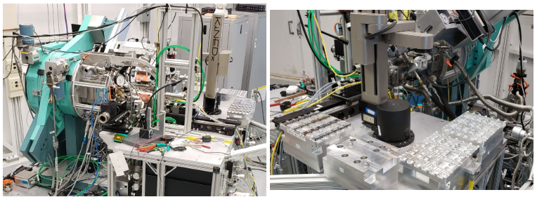
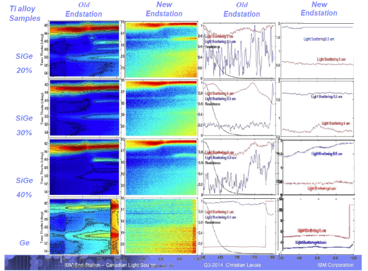
IBM Endstation: In-Situ Rapid Thermal Annealing
This endstation can operate at two fixed photon energies: 7159.2 eV (1.73184 Å) with Si(111), or 13691.0 eV (0.90560 Å) with Si(311). Typical operation is at 7.1 keV, except some circumstances where greater penetration through high Z elements is required.
This endstation is highly specialized for rapid thermal annealing experiments on metallic thin films and multilayer structures under controlled atmospheres. It can perform simultaneous X-ray diffraction, four point probe resistivity measurements, and surface roughness measurements on thin films during rapid annealing, up to 1100°C. It is generally for industry use but has been made available for specific user experiments. Please discuss your IBM endstation proposal with beamline staff before submitting.
The WLE beamline has three endstations supporting the following techniques,
- High-Resolution Powder X-ray Diffraction
- SAXS/WAXS
- IBM Endstation
Scroll down this page to find out more! We offer a mail-in access option for all the techniques.
Please contact Adam Leontowich for questions related to the WLE beamline.